Signals and Systems
Function transformations:
h(t) to other forms:
Before making convolution in time domain, we need to transform impulse response function into the required format:
Example 1:
We have \(h(t)=s(T-t)\).
We will make convolution as \(z(t)=r(t)*h(t)=\int_0^t r(\tau)h(t-\tau)d\tau\).
Impulse response should pass these stages:
\(h(t)=s(T-t)\)
\(h(\tau)=s(T-\tau)\)
\(h(-\tau)=s(-T+\tau)\)
\(h(t-\tau)=s(t-T+\tau)\)
Substitute into \(\int_0^t r(\tau)h(t-\tau)d\tau=\int_0^t r(\tau)s(t-T+\tau)d\tau\)
Example 2:
We have \(h(t)=u(t)\).
We will make convolution as \(\int_0^t x(\tau)h(t-\tau)d\tau\).
\(h(t)=u(t)\)
\(h(\tau)=u(\tau)\)
\(h(-\tau)=u(-\tau)\)
\(h(t-\tau)=u(t-\tau)\)
Then substitute.
Convergence of the Fourier Series
Periodic signals can be represented by Fourier series under certain conditions:
- Energy of the signal over one period should be finite.
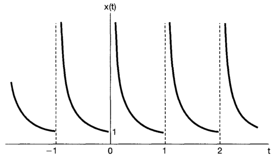
For example, the signal violates this condition:
\(x(t)=\frac{1}{t}\), Period: \(0< t\leq1\)
- Signal must have finite number of maxima and minima in a finite time interval.
- Signal must have finite number of discontinuity in a finite time interval.
Telecommunications
Error Probability Performance
Bit error probability of equally likely, binary signals:
\(P_B=\int_{\frac{a_1-a_2}{2\sigma_0}}^\infty \frac{1}{\sqrt{2\pi}}e^{-\frac{1}{2}(u)^2}du=Q(\frac{a_1-a_2}{2\sigma_0})\)
In the nominator of argument of \(Q\), we see voltage difference (square root of power or square root of energy) of signals.
\(p^2=\frac{v^2}{R}\), \(power=\frac{Energy}{time}\)
\([\frac{volt^2}{ohm}]=[watt]=[\frac{Joule}{sec}]\)
\([\frac{volt}{ohm}]=[\frac{Coulomb}{sec}] \Longrightarrow [\frac{volt*sec}{ohm}]=[Coulomb] \Longrightarrow [\frac{volt^2*sec}{ohm}]=[volt*Coulomb]=[Joule]\)
Taking the square root of Joule gives not only volt but \([\frac{volt*\sqrt{sec}}{\sqrt{ohm}}]\). Since in the questions, both transmitted signals and noise values are given, the \(sec\)s (maybe \(ohm\)s (?)) cancel each other and no need to consider.
The nominator is the difference between signals in terms of voltage.
-
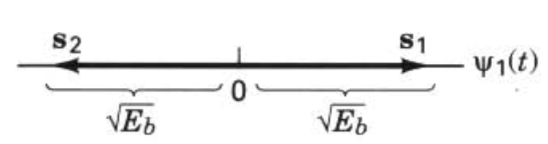
For antipodal signals, the difference is \(2*\sqrt{E_b}\). For \(s_1(t)\), \(a_1=\sqrt{E_b}\).
For \(s_1(t)\), \(a_2=-\sqrt{E_b}\).
\(a_1-a_2=2*\sqrt{E_b}\).
\(E_b\): energy of a bit
The variance of noise is given as \(\frac{N_0}{2}\) in general.
\(Q(\frac{a_1-a_2}{2\sigma_0})=Q(\frac{1}{2}\frac{2*\sqrt{E_b}}{\sqrt{\frac{N_0}{2}}})=Q(\sqrt{\frac{2E_b}{N_0}})\)
Or equivalently, \(Q(\frac{a_1-a_2}{2\sigma_0})=Q(\frac{1}{2}\frac{\sqrt{E_d}}{\sqrt{\frac{N_0}{2}}})=Q(\sqrt{\frac{E_d}{2N_0}})\)
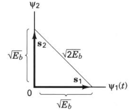
- For orthogal signals, the difference is \(\sqrt{2*E_b}\).
\(Q(\frac{a_1-a_2}{2\sigma_0})=Q(\frac{1}{2}\frac{\sqrt{2E_b}}{\sqrt{\frac{N_0}{2}}})=Q(\sqrt{\frac{E_b}{N_0}})\)